A Reporter’s Guide to Excel

Reporters use Microsoft Excel to analyze data to look for trends, anomalies and story ideas. Databases are full of information broken down into rows and columns. This guide will teach skills that are needed to clean and analyze databases to extract information for story use. Remember, there are stories in the data.

Use this guide as an introduction to the Excel concepts you’ll find most helpful in your reporting, and remember to be patient. Many Excel tricks require some practice, but you’ll see the payoff quickly. And if you make a mistake, just hit “control+z” to undo a step.

Accompanying this guide is a set of spreadsheets that you can use to practice the skills you’re about to learn. The examples in this guide mirror the examples in the spreadsheets.

Get the Data

The first step is to get the data. State laws vary, but a basic request should detail specifically what is needed and the time frame sought. Also, always request the information in electronic format, such as Excel. And make sure to request the record layout, which will define the information in each column. Some column headers consist of abbreviations, and you don’t want to guess them.

Basic Excel Organizing Tools

Excel is made up of columns and rows. Columns have letters and are vertical. Rows have numbers and are horizontal. Consider this the latitude and longitude of data mining.

Excel allows you to manipulate data in time-saving ways, but it helps to know the basic editing and organizing functions to quicken the pace of your analysis. In some cases, applying a simple edit to your cells can eliminate the need for more involved formulas. In other cases, you’ll want your data organized in certain ways before advancing to the formulas we’ll explore in this guide.

Sort: This is the fastest way to rank data in a column. The sort function works for text and numbers. At its most basic, the Sort option allows you to organize rows of data in one or more columns numerically or alphabetically. To do a quick sort in Excel, right click anywhere in the column you want to sort. [See example ‘SORT’ below]

Sort & Filter

To sort by more than one level, do a customized sort. Under the home tab, click on Sort & Filter and then Custom Sort.

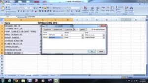
Custom Sort Menu

Filter

The Filter is sorting on steroids. In addition to organizing rows in one or more columns by their alphabetical or numerical order, this function allows you to limit the data on display for more targeted analysis. For example, if you have a district employee spreadsheet and one of the columns identifies the employee type (principal, teacher, librarian, etc.), you’ll be able to use the Filter function to select as many or as few types of employees as your analysis requires. To turn on the filter, click on the Home tab and go to Sort & Filter. Click on filter, and you will see the pull down tabs on the column headers. For more in-depth filters, click on the filter tab and go to “date filters” or “text filters.”

Format Cells Using ‘Home’ Tab Features

To format a cell or column, right click on the cell or highlight the column. Go to Format Cells. Under the Number tab, you can specify the format of the cell as general, text, a number, a date, currency, etc., or customize it. The Alignment tab allows you to align text, wrap text, merge cells, etc. You can add a border to your spreadsheet under the Border tab. You’ll want to format your cells regularly as some formulas call for text, while others call for numbers. Knowing what the formulas call for is part of the fun of Excel!

Freeze Panes

To freeze the header row, got to the View tab and click on Freeze Panes. (Mac users follow these steps.) Three options allow you to freeze the top row or the first column, or to designate a combination of top row/column to freeze. As you become more acquainted with Excel, this function will likely stand out as one of the most useful. In spreadsheets with hundreds of rows and dozens of columns, it’s hard to keep track of what each row or column represents — unless, of course, the header (name) of each row or column stays in place as you scroll through your spreadsheet. Notice in the example below that the top row is numbered “1” but the following rows start at number “1583.” As you scroll through the data, the “freeze pane” (in this case, the top row) stays in place so that you don’t lose track of the headers.

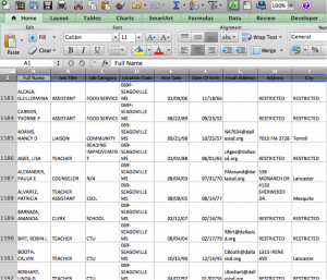
Freeze Row

Transpose

This function allows you to flip columns into rows and vice versa in Excel. Here is the easiest way to transpose information: Highlight and copy the cells you want transposed. Once copied, go to the cell where you want your transposed information to appear. Right click on the empty cell and click on Paste Special in the menu. Next, check the transpose box near the bottom and hit OK.

Add/Delete rows and columns

To add rows and columns, highlight the area where you want the new rows or columns. Right click, and click Insert. If you want to add five rows/columns, then highlight five rows/columns and then click Insert. To delete rows/columns, highlight the rows/columns to delete. Then, right click and hit Delete.

Adjust column width

There are a couple of ways to adjust the column width. The easiest way is to left click on the line and drag it to where you want it. You can also highlight the row or column, right click, and then click Column Width. Enter the desired column width and hit OK.

Key Functions

A good starting tip with functions is knowing what formula was used to arrive at an answer. If you see a number in a cell, click on it to see if that number was derived from a mathematical function, like the ones you’ll learn about in this section. This is also good to keep in mind as you gather more information through formulas and want to double-check how you arrived at those figures or calculations.

Addition

To add two cells, select the cell in which you want the total to appear and type: =b2+b3.

To add a column of numbers use: =sum(b2:b10)  [See Example 1]

You can either type out the range “b2:b10” or move your cursor to select the part of the column you wish to apply to your function, in this case the ‘sum’ function. Practice dragging your cursor along the cells you want to add; you’ll notice that Excel applies a light color to the cells you’re pulling into your equation. This trick can be applied to nearly all functions.

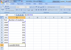
Example 1 | Sum

To subtract

=b3-b2 (Which in Example 1 above would result in 432-267)

Median

The middle number in a group of numbers. For example, the median of 2, 3, 3, 5, 7 and 10 is 4. Use the median instead of average when numbers in a set differ greatly. For example, finding the median salary for the Dallas Mavericks players would be more useful than finding the average salary, as the star player makes millions more than all other players and his salary would skew the data. Using Example 1, here’s how you find the median: =median(b2:b10)

Mode

The most frequently occurring number in a group of numbers. For example, the mode of 2, 3, 3, 5, 7, and 10 is 3. Mode can be used to highlight important information in data, such as pointing out that the majority of teachers make $47,000 a year. Using Example 1, here’s how you find the mode: =mode(b2:b10)

Average

The formula to find the average is =average(b2:b10)

Maximum

To find the maximum number in Example 2, the formula is =max(a2:a23)  The max number is 22.

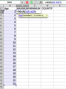
Example 2 | Max

Minimum

To find the minimum number, the formula is =min(a2:a23)

Countif

Counts the number of cells that meet the criteria that you specify. In Example 2, find the number of people over age 20 with this formula (note the quotation marks): =countif(a2:a23, “>20”). The answer is 2. The countif formula also can be used for text, such as the number of times a name appears in a column.

Percentage

Calculating percentages in Excel. Example 3 shows how to find the percentage that each county in Texas constitutes of the state. The formula is =b242/b257 with b257 being the total that you’d use as your denominator. Notice that in the example you first needed to add all the values in the range in column B, where it says “total.”

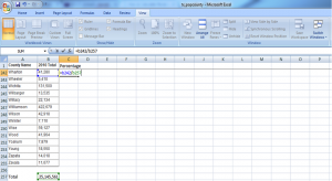
Example 3 | Percentage

Anchoring

Instead of writing the percentage formula for each cell, use the copy function by dragging or double-clicking. But you will get error messages in those cells unless you anchor the denominator, or hold it constant. Do this in Example 3 by adding a dollar sign to the formula: =b242/b$257

Per Capita

Allows you to make apples-to-apples comparisons for entities that may not be of equal size. Example 4 shows the number of property crimes per 100 people at select universities: =(H2/B2)*100. If you wanted to represent the data per 1,000 people, you’d do this: 54,942/1,000=X; 378/X.

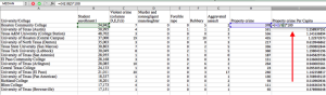
Example 4 | Per Capita

Percent Change

Finding the percentage differences between two numbers. In Example 5, use =(b2-c2)/c2. An easy way to remember this formula is to think of “NO” with an extra “O”  =(New number-Old number)/Old number. In Example 5, using the formula, we see the number of forcible rapes declined by about 10.8 percent from 2004 to 2008. Why decline? Because the formula spits out a negative value (-.1080118694). Another way of remembering percent changes is by relying on fractions you know well, like those with the numbers 3 and 4. Went from 3 to 4? You grew by a third [(4-3)/3]. Dropped from 4 to 3? You declined by a quarter [(4-3)/4], which is another way of saying you grew by [(3-4)/4], or negative ¼.

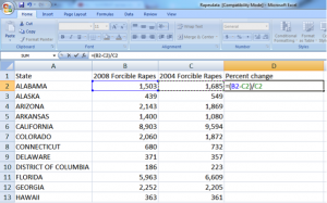
Example 5 | Percentage Change

If

The “If” function allows you to determine if a condition is true or false according to your own parameters. Like many other formulas, this one is executed in a new column. For example, if your story calls for determining the proficiency levels of various schools, and you have the raw scores but also know the cut-off points for each achievement level, you can create an If statement that inserts a new column whether the achievement level was at-or-above proficient or not. The following example uses a more simple If statement =if(a2<b2,“Too much”, “OK”)   [See example 11]

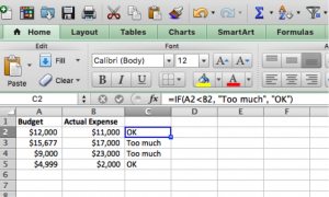
Example 11 | IF

Sum If

The sumif formula allows you to sum information fitting a particular condition. The following formula will sum the number of property crimes committed in cities with a population over 15,000:  =sumif(b2:b8,“>15000”,c2:c8)  [See Example 12]

The formula breaks down like this:

b2:b8 is the population of each town
“>15000” seeks information for cities with populations over 15,000 (notice the quotes)
c2:b8 is the range for the property crime data

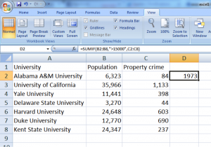
Example 12 | SumIf

Sum Ifs

This is a supercharged Sum If that allows the user to find data with added precision. The formula is somewhat different than Sum If, but the logic is similar. Say a story calls for property crime for universities in cities of a certain size, organized by whether the school is private or public. By adding that new variable — public or private — a new formula is in order. Here’s what to do to find the number of property crimes of public universities in towns that have a population of more than 15,000: =sumifs(d2:d8,c2:c8,”>15,000″,b2:b8,”Public”) [See Example 13]

The formula breaks down like this:
d2:d8 is the range for the property crime data
c2:c8 is the population of each town
“>15000” seeks information for cities with populations over 15,000 (notice the quotes)
b2:b8 is the range that identifies whether the school is public or private
“Public” seeks information only for public schools